Social dynamics of bluetooth speakers

A mathematical model of who turns on their bluetooth speaker at the beach.

Say you’re at a park or a beach. How many people will have bluetooth speakers on? It seems to me there are three types of people:

• The main characters always turn on their speakers regardless of what anyone else is doing.

• The haters never turn on a speaker, no matter what.

• The normies turn on a speaker if a large enough fraction of other people are doing the same.

There are different reasons normies might behave this way. Some might like to listen to music but—bless them—worry that it’s rude, so they won’t do it unless others have normalized the behavior. Some might not want to listen to music, but at , they’ll turn on a speaker defensively so they can listen to their own music instead of yours.

For our purposes, none of this matters. All we need is that everyone has a threshold.

So, our question: If you put a mix of these different types of people together, what happens?

Model 1

Each person has some threshold t at which they’ll turn on their speaker. Assume:

• A fraction A of people always turn on their speaker (t=0).

• A fraction B of people never turn on their speaker (t=1.01).

• The rest have different thresholds, equally distributed from 0 to 1.

Say we throw all these people together into a silent park. What will they do? Well, a fraction A will immediately turn their speakers on. That will induce more people to turn theirs on, and so on. But how does it end? If we had started with everyone having speakers on, would we get the same result?

To formalize this, define:

    p(t) = the fraction of people with a threshold of t.

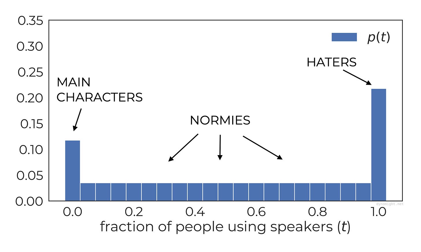
For the sake of illustration, assume A=0.1 and B=0.2. Then the distribution of thresholds (quantized to intervals of 0.05) looks like this:

This plot is intuitive, but it’s not very helpful to understand the dynamics of the model. Instead, we need to introduce a slightly different object:

    F(t) = the fraction of people with a threshold of t or less.

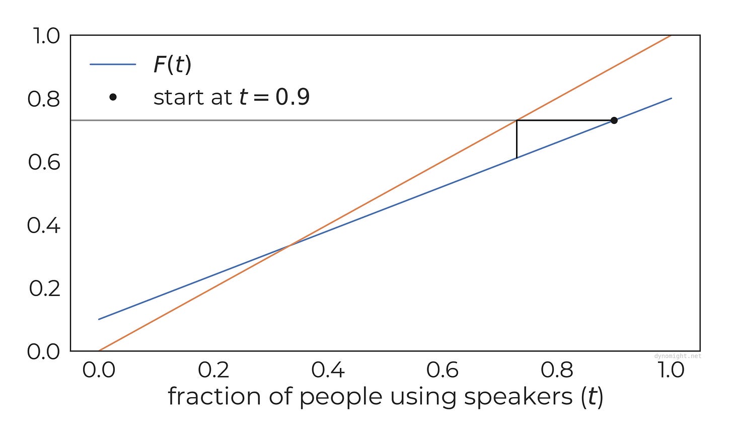
Technically F(t)=p(T≤t) is a “cumulative distribution function” but never mind. Here’s what it looks like:

Since 10% of people always turn on their speakers, F(0)=0.10. And since 20% of people never turn on their speakers, F(1)=0.80. Between that, it’s a straight line.

OK! Let’s try this model out. Assume that people are in a park, and 90% are initially using speakers. What happens next?

Well, if everyone sees 90% of people using speakers, how many will use one themselves? The calculation we need is that F(0.90)=0.73. We can picture this as a horizontal line in the following graph. (This also shows the identity curve t=t, which will soon be relevant.)

What does this mean? The following statements are equivalent:

• F(0.9)=0.73

• 73% of people have a threshold of 0.9 or less.

• When this group of people observes 90% of themselves using speakers, only some will feel it is appropriate to use a speaker themselves. How many will feel that way? 73%

So, after everyone’s had a chance to look around and decide what to do (in the next “time step”) 17% of the people will turn off their speakers. Geometrically, this is what we get if we “bounce” the above horizontal line off the t=t curve.

So now we’re at the next time-step, and 73% of people are using speakers. Well, time keeps moving forward and the process repeats. Since F(0.73)=0.611, if this group observes 73% of people using speakers, only 61.1% will use one themselves. So even more people turn their speakers off.

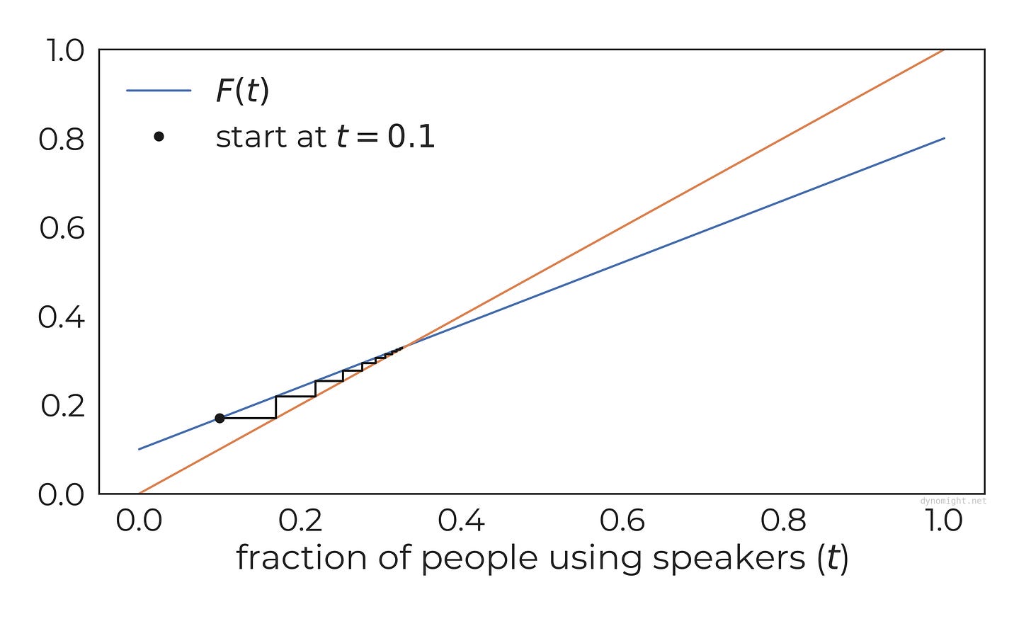
We can run this simulation forward in time as many steps as we like. Eventually, things seem to converge to around t ≈ ⅓.

What if we had started with only 10% of people with speakers on instead? We’d have the opposite situation, where some people would turn on their speakers, and that would induce others to do the same. But we still end up at t ≈ ⅓.

Mathematically, we can show that this is the unique solution. For this model, you can show that F(t) takes the form (if you don’t like math it’s fine to skip these equations)

    F(t) = A + (1-A-B) × t.

A fraction t will be an equilibrium if and only if F(t) = t, i.e. where the two curves cross. It’s not hard to show that the unique equilibrium is

    t = A/(A+B).

This is natural: The higher the fraction of main characters relative to the number of haters, the larger the fraction of people who end up with speakers on.

Simple, right? Yes, but things get weirder with some seemingly innocuous changes to our modeling assumptions.

Model 2

Again, suppose there are three different kinds of people.

• A fraction A of people always turn on their speaker (t=0).

• A fraction B of people never turn on their speaker (t=1.01).

• The others have different thresholds.

The only change is the distribution of thresholds for people in the last group. Rather than being uniformly distributed, we let’s assume they have a threshold near t=0.25, but with some random noise added.

Technically, we assume normies have a threshold that comes from a Normal distribution (ha) with a mean of 0.25 and a standard deviation of 0.05. (OK, technically it’s a truncated Normal distribution, but we’re only truncating 5 standard deviations out, and anyway simmer down there, this is a blog post.)

Anyway, here’s the corresponding F(t).

Look at that—there are three solutions to the equation F(t) = t. These equilibria turn out to be:

• t ≈ 0.101. In this solution, the main characters all have their speakers on and basically no one else

• t ≈ 0.195. In this solution, it’s the main characters and a bit less than half of the normies

• t ≈ 0.8. In this solution, it’s almost everyone except the haters.

That’s interesting, but let’s try simulating it. Here’s what happens if we start at t = 0.185:

Even though we’re starting just below middle equilibrium, the fraction of people using speakers quickly drops down to main characters only.

Meanwhile, here’s what happens if we start at t = 0.205, just on the other side of the middle equilibrium:

Now, the fraction of people using speakers quickly increases to everyone except the haters.

Even though there’s an equilibrium at t ≈ 0.195 in this model, it is unstable— any tiny random perturbation results in a completely different solution.

The standard analogy for unstable equilibria is:

• A marble in a bowl is in a stable equilibrium.

• A pencil balanced on its point is in an unstable equilibrium.

How can you tell if an equilibrium will be stable or not? For our types of models, there’s a simple geometrical answer: Remember, every equilibrium is a solution to the equation t=F(t), i.e. point where the F(t) curve crosses the t=t curve. Now:

• If the F(t) curve crosses “from the bottom to the top”, with a more vertical slope, that will be an unstable equilibrium.

• But if it crosses “from left to right”, with a more horizontal slope, it will be a stable equilibrium.

So, weirdly, instead of having a single equilibrium in the middle like in the first model, our second model has two extreme stable equilibria, and which one people end up at depends on the initial conditions.

Weird, but not weird enough. Let’s keep going.

Model 3

Yet again, suppose there are three different kinds of people.

• A fraction A of people always turn on their speaker (t=0).

• A fraction B of people never turn on their speaker (t=1.01).

• The others have different thresholds.

And again, our only change will be to the distribution of people in the third group. Now, half of them have a threshold near 0.25 with some noise, while the other half have a threshold near 0.65. (Perhaps those near 0.25 are those who want to use speakers and so they do as soon as it’s normalized, while those near 0.65 are “defensive” speaker users.) In both cases, we assume the noise is Normal with a standard deviation of 0.05.

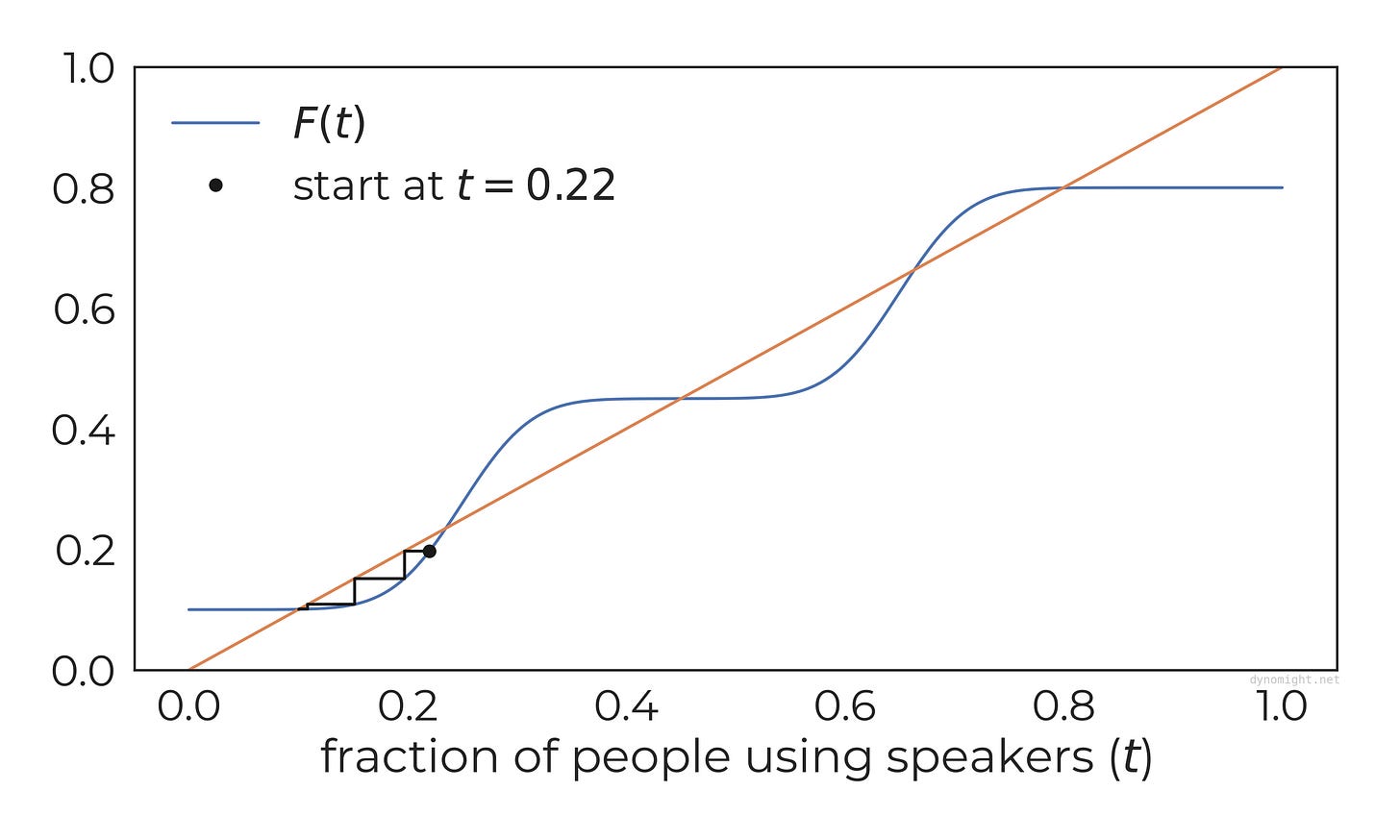
Here’s what the corresponding curve F(t) looks like:

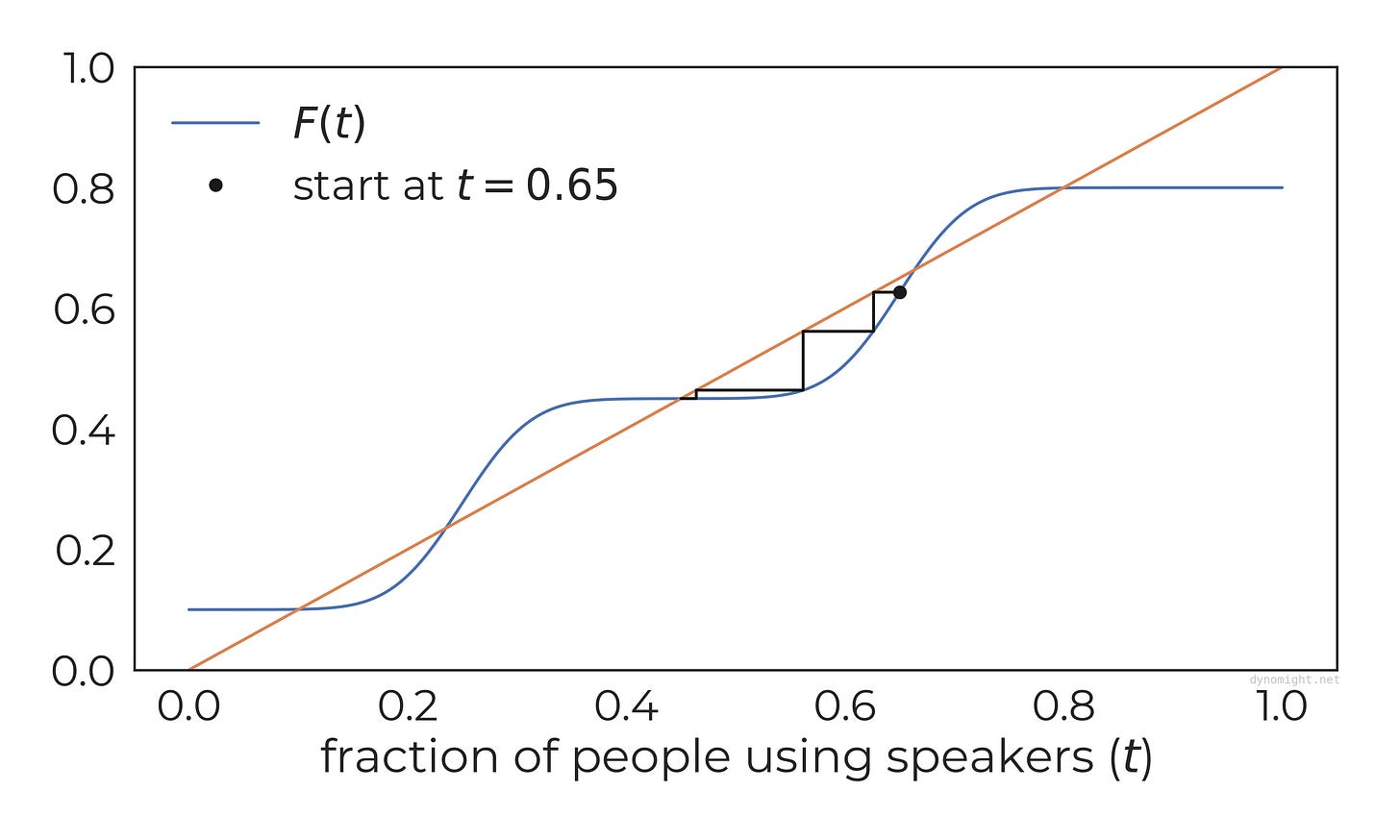
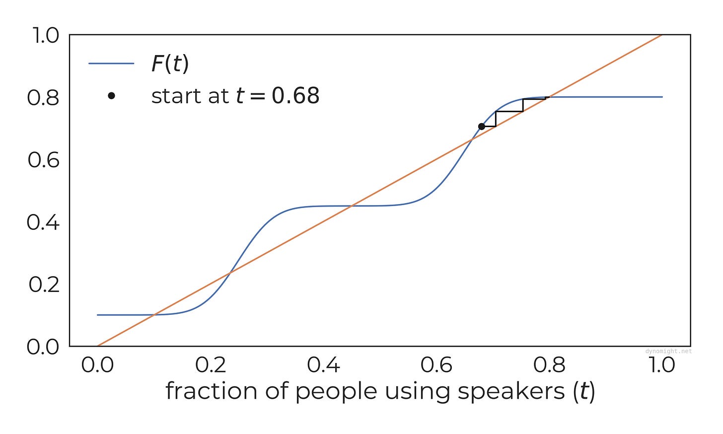
Five equilibria! Depending on where we start the simulation, Many different things can happen. Here are four examples:

Of the five equilibria (places where F(t)=t), three are stable and two are unstable. This follows from the same rules from above: When F(t) has a steeper slope than t=t at the crossing, it produces an unstable equilibrium, while if it has a gentler slope, it is a stable equilibrium.

Dynamics

Which of these corresponds to real life? Eh, I’m not sure.

What we’ve seen is that with relatively modest changes to the model, you can have vastly different solutions. This is even worse than the above examples might suggest. Suppose we took model 3, and instead of giving people thresholds near 0.25 and 0.65, we used 0.25 and 0.75. It turns out that this means the top two equilibria disappear!

So, unfortunately, these models depend on the precise details of what thresholds different people have. Since it’s hard to be confident about what that is, it’s hard to be confident in the predictions of these models.

However, if I had to guess… I suspect that in real-life, bluetooth speaker usage usually just has one stable equilibrium. That’s because I suspect that most people are either “main characters” or “haters”—they aren’t influenced by other people much at all.

Why does this matter? Well, suppose that 25% of people always use a speaker, 50% of people never use a speaker, and the other 25% of people have some threshold in the middle. Now, depending on how those thresholds are distributed, you get different functions F(t). They could in principle be anything, but they have to start at F(0)=0.25 and end at F(1)=0.50. Here are four randomly generated options:

See the issue? If there aren’t many normies, then the curve F(t) will be mostly horizontal, which makes it hard to get multiple crossings.

So, multiple equilibria in bluetooth speaker usage are possible but you’d need:

• a lot of people who change their speaker usage in response to what others are doing, and

• that those people have thresholds that are fairly clustered (to cause a sudden upward lurch in the F(t) curve), and

• the value where the thresholds cluster happens to be situated so that the upward lurch in F(t) causes a new crossing with the t=t curve.

Could happen, but not all that likely.

Advice

Beyond the difficulty of controlling the equilibrium, none of this says anything about the average happiness of all people. Given the difficulty of estimating that, my advice is—if you have a bluetooth speaker, use it. Use it at the park, the beach, on public transportation. Use it while hiking. Do this even if you’re alone. And remember, it’s paramount that you spread out from anyone else that’s also using a speaker: If all the bluetooth captains were to carelessly cluster together, that might leave the occasional pocket of public space where someone could exist without enjoying the latest innovations in auto-tune hyperpop electro-maximalism, and that, that would be a tragedy.

---

Update: See also Eric Neyman’s Social behavior curves, equilibria, and radicalism. This type of model is known in sociology as a “threshold model”. For example, Granovetter (1978) includes this figure: