Life with hazard ratios

How to discount your expectations

dynomight.net/hazard-ratios

If you read anything about health or longevity, you’ll soon find yourself in a world of hazard ratios. Some study might say that eating more fiber might change your risk of dying by a factor of HR = 0.90. Another might say that occasional smoking might change it by HR = 1.30.

But how much should you care about that? Is HR = 0.90 or HR = 1.30 a lot? What if you don’t want to eat more fiber? What if you like smoking?

Instead of staring at a ratio^[1], a more sensible thing to do is think about life expectancy.^[2] But is it possible to convert a hazard ratio to a change in life expectancy? You might reason as follows: Baseline life expectancy is around 75 years. And HR = 0.90 corresponds to a 10% decrease in mortality. So perhaps that hazard ratio corresponds to something like 7.5 extra years of life expectancy?

Unfortunately, that’s completely wrong. To see why, imagine that humans only die by playing Russian roulette. They start playing this once per day at the age of 75, with a revolver containing two bullets and six chambers. If you were to remove one of those two bullets, that would drop the person’s risk of death by HR = 0.5. (One bullet versus two.) But life expectancy would barely change, because even with just one bullet, almost nobody would survive for any significant amount of time past 75.

For contrast, imagine again that humans only die via Russian roulette, but now they do this once per day from birth with a revolver with 2 bullets and 54,786 chambers. (Newborns emerge and instinctively reach for this gigantic gun.) You can show that these people also live 75 years on average. But now, if you remove one of the bullets, life expectancy doubles, because when someone is spared, it takes a long time before they get unlucky again.^[3]

Neither of those is a good model for humans. We’re somewhere between the two, with heart disease and so on instead of revolvers and risks slowly rising as we age instead of suddenly starting at age 75 or staying constant throughout life. But you get the point: If you want to convert a hazard ratio for some intervention to a change in life expectancy, the impact depends on how “spread out” baseline mortality risk is over time. Baseline life expectancy is simply not enough information.

That’s one problem. Here’s another: What even is a hazard ratio? The technical definition is something like:

The hazard ratio at a given time is the rate of an event in the treatment group divided by the rate of that event in the control group.

Hazard ratios are often confused with their more beloved siblings, relative risks. Say you run a trial for 10 years and at the end, 10% of the control group died and 8% of the treatment group. Then the relative risk is RR = 0.8, nice and simple. But relative risks have problems, most notably that if you run a long enough trial, then no one will be alive at the end no matter the intervention, meaning RR = 1.0. That’s not helpful. Intuitively, you can think of the hazard ratio at age 40 as sort of like the relative risk for people between the ages of 39.99 and 40.01.

In real life, interventions have different hazard ratios at different ages. Chemotherapy tends to have better results in younger patients who are more able to endure the side-effects. Having a slightly higher BMI (25-30 rather than 20-25) is associated with an increased risk of mortality in young people, but a decreased risk in the elderly. You may remember from 2020 that COVID’s mortality risk had a different age curve than baseline mortality, meaning the hazard ratio of getting COVID was different at different ages.

This is important, because hazard ratios at different ages have different impacts on life expectancy. A hazard ratio of 0.9 at age 80 prevents more deaths than at age 20, because baseline mortality is higher at 80. But at the same time, if you save the life of a 20 year-old, they have more years in front of them. Beyond that, the hazard ratios at different ages interact: If some intervention decreases mortality at younger ages, that allows more people to reach older ages, increasing how much hazard ratios matter at older ages.^[4]

If we knew the hazard ratio at all ages, we could account for those dynamics. But we don’t, because when estimating hazard ratios, people almost always assume that the hazard ratio is constant.^[5] We’re quasi-forced to do this because there’s not enough data to estimate a whole time-series of ratios. That’s why papers contain single numbers like HR = 0.90.

So even though Intervention A (say, more fiber) and Intervention B (say, light jogging) might have the same hazard ratio in a paper, those numbers could be the product of different underlying age-dependent effects, meaning those interventions could conceivably lead to vastly different changes in life expectancy.

So is this all hopeless? Are single hazard ratio numbers just too far removed from what we care about to tell us anything meaningful?

Surprisingly, no. It’s mostly OK. If we were a different species, it might be hopeless. But for modern humans in rich countries, mortality happens to be distributed in a way that produces a sort of lucky coincidence: When people estimate constant hazard ratio numbers, they’re implicitly sorta-kinda taking a weighted average of hazard ratios at different ages. And those weights happen to (sorta-kinda) reflect how much changes in mortality at different ages change.

So, I will argue, even if the true intervention has a varying effect, it’s sorta-mostly OK to just take a hazard ratio from a paper and convert it to a change in life expectancy using this curve:

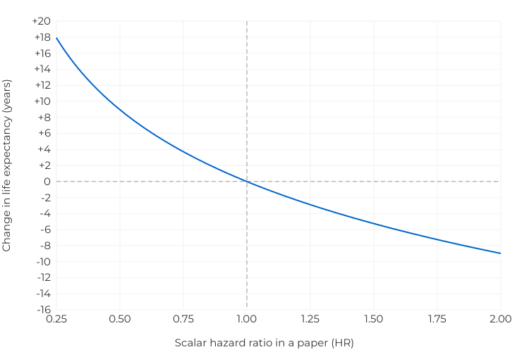
If a paper showed that eating more fiber produces a hazard ratio of HR = 0.75, that corresponds to an increase of around 3.7 years. If a paper says that occasional smoking produces a hazard ratio of HR = 1.25, that corresponds to a decrease of around 2.9 years.

This isn’t exact. If the intervention is better (or less bad) for older people this will tends to overestimate the increase (or underestimate the decrease) in life expectancy. If the intervention is worse (or less good) for older people, it will tend to underestimate the increase (or overestimate the decrease) in life expectancy. But as long as the hazard ratio doesn’t vary too much by age, it’s probably not off my more than around 30% in either direction.

The easy case

Say there’s some intervention (eating more fiber or whatever) that multiplies your risk of dying at age t by a factor of HR(t). Then it can be shown that this changes life expectancy by approximately

ΔL ≈ ∑ₜ ΔHR(t) × P(t) × L(t).

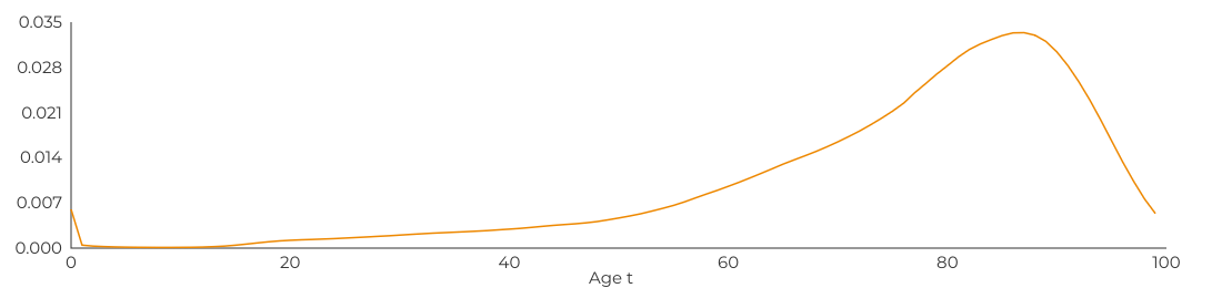
Here, P(t) is the baseline probability of dying at age t. For males in the United States, it looks like this:

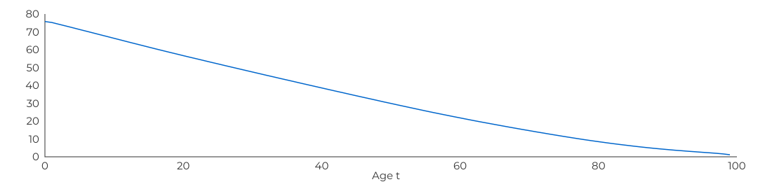
Meanwhile, L(t) is conditional life expectancy at age t. That’s the average number of additional years left for someone who reaches age t. For males in the United States, it looks like this:

Finally, ΔHR(t) is the decrease in hazard at age t. You can think of that as just ΔHR(t) = 1 - HR(t). Though if you’re OK with logarithms, there’s a somewhat better approximation that uses logarithms, which I’ve quarantined in a footnote.^[6]

Let’s start with the easy case. What if your intervention has the same effect on mortality at all ages, so HR(t)=HR is just a constant? Then, the above equation simplifies into

ΔL ≈ ΔHR × l,

where

l = ∑ₜ P(t) × L(t).

This makes sense! Again, P(t) is the baseline probability of dying at age t and L(t) is conditional life expectancy at age t. These are constant, so when you add them up, l is just a number. For males in the United States, it happens to be 12.93 years. This quantity has a specific meaning: The average remaining life expectancy for US males when they die. That sounds a bit odd, but think of picking a random death and asking how many additional years people who reach that age live on average. That number is 12.93 years.

So, if an intervention has a constant hazard ratio, the mean change in life expectancy for US males is just

ΔL ≈ ΔHR × 12.93 years.

Now we’re getting somewhere! If you prevent a fraction ΔHR of deaths, then you increase life expectancy by ΔHR times 12.93 years.

Now remember the naive calculation we started with: Life expectancy for US males is 75.8 years. You might hope that if eating more fiber drops your risk of death by 10%, that would save 7.58 years. Sadly, the above equation says that a 10% drop in risk only increases life expectancy by around 1.293 years—only 0.17 times as much.

This is essentially the observation Keyfitz made in his 1977 paper, “What Difference Would It Make if Cancer Were Eradicated?” Cancer is responsible for 18 percent of deaths, so does that mean eradicating it would increase lifespan by 18 percent, or around 13.6 years? Nope, Keyfitz says, it’s only 2.3 years.

If a cure for cancer were discovered and made available today, 350,000 cancer deaths would be avoided in the next year. The overall death rate would be lower by nearly 18 percent. If the cure were quick and inexpensive, a large fraction of the country’s hospital beds and medical personnel would be released for treatment of other ailments. Patients would be spared untold suffering. Such an implicit analysis underlies government proposals for eradication of cancer. The argument is sound for first effects on mortality but wholly misleading for the long term.

The first effects would soon be offset by more mortality from diseases other than cancer. As a result of the cancer cures, the population would include a higher proportion of people subject to other causes of death. […]

At the extreme, it might be said that everyone dies of something sooner or later, so that, when the effects of the eradication of cancer had shaken down, the same number of deaths would occur as before, and the only benefit would be the substitution of heart and other diseases for cancer. A cure for cancer would only have the effect of giving people the opportunity to die of heart disease.

Cheerful stuff! We can also write our approximation in terms of baseline life expectancy as

ΔL ≈ ΔHR × 0.17 × 75.8 years,

which makes explicit that 12.93 years is only 0.17 times as large as a naive estimate using baseline life expectancy. The discount factor of 0.17 is sometimes called the “Keyfitz entropy”. You can think of it as measuring how close some population is to playing Russian roulette with 2 bullets in 6 chambers starting at age 75 (a discount factor of just above 0) and playing Russian roulette from birth with 2 bullets and 54,786 chambers (a discount factor of 1.0). It’s typically around 0.15 in rich countries today, though it was historically much higher.

Keyfitz entropy is also much higher in other species like mice (perhaps 0.45). You could argue that this explains why nothing that increases lifespan in mice ever translates to humans. Say caloric restriction or whatever produced the same constant hazard ratio in mice and humans. Then it’s mathematically guaranteed that the percentage increase in life expectancy will be three times smaller in humans, because Keyfitz entropy is three times smaller in humans. It’s harder to increase life expectancy when the baseline mortality distribution is more compressed.^[7]

But that’s all assuming the hazard ratio is the same at all ages. Which it surely isn’t.

The interesting case

Here again is our equation for the change in life expectancy in response to taking some action that changes the risk of mortality at age t by a factor of HR(t):

ΔL ≈ ∑ₜ ΔHR(t) × P(t) × L(t),

Basically, for each age t, we multiply together three numbers:

1. ΔHR(t) is the decrease in the chance of dying at age t as a result of whatever intervention you’ve made (e.g. eating more fiber). This reflects that larger decreases in risk lead to larger increases in life expectancy.

2. P(t) is the baseline probability of dying at age t. This reflects that the hazard ratio is a ratio, so you prevent more deaths when you apply that ratio to ages where the baseline rate is higher.

3. L(t) is conditional life expectancy at age t. This reflects that you miss out on more years of life if you die when you’re young.

Now notice: The impact of a change ΔHR(t) at age t is the product of the baseline risk of death P(t) and remaining life expectancy L(t). So what really matters is their product, P(t) × L(t):

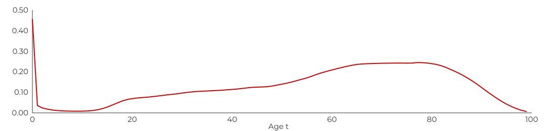
This shows how sensitive life expectancy is to changes in hazard ratios at different ages. It would be nice if this were constant. Then, the shape of HR(t) wouldn’t matter at all, only the average value. That’s not quite true, but it’s not terribly far from being true.

An equivalent way of writing our equation for the change in life expectancy is

ΔL ≈ avg(ΔHR) × l,

where l is still mean “life expectancy at death” (12.93 years for US males) and avg(ΔHR) is the average change in hazard, weighted by the P(t) × L(t) sensitivity curve at different ages.^[8] While that sensitivity curve isn’t constant, it’s not too curvy, either. Intuitively, it gives a lot of weight to ages between 50 and 90, somewhat less weight to ages between 20 and 50, and little weight to other ages.^[9]

So that’s not too bad. But let’s remember our original problem: You see some number like HR = 0.90 in a paper, and you want to convert it to a change in life expectancy. If the true underlying hazard ratio were constant, then there’s no problem. But if it’s not constant, then what does that HR = 0.90 number even mean?

Numbers in papers

Unfortunately, you almost never get to see the underlying time-dependent HR(t), because there’s almost never enough data to estimate it. So it’s almost never possible to compute the weighted average avg(ΔHR). In reality what you have is probably a single number in a paper. Let’s call that number est(HR). The obvious thing to do would be to plug the change into the above equation in place of avg(ΔHR) and approximate the change in life expectancy as

ΔL ≈ est(ΔHR) × l.

Again, you can just think of est(ΔHR) = 1-est(HR) as being the estimated reduction in hazard. Although, again, I’d prefer you use logarithms if you’re OK with logarithms.^[10] So the question is: Will that be accurate? How close are est(ΔHR) and avg(ΔHR)?

Well, how do people actually estimate those scalar hazard ratio numbers in papers? Somehow, they’re aggregating together information about hazards at different ages into a single number. But how? Well, it’s complicated. But if there’s a lot of data, you can show that the estimated scalar hazard ratio is approximately^[11]

est(HR) ≈ Πₜ HR(t)ᵖ⁽ᵗ⁾.

That is, the estimated hazard ratio is the geometric average of age-dependent hazard ratios, weighted by the probability of dying at each age. It follows^[12] that the estimated change in hazard is approximately

est(ΔHR) ≈ ∑ₜ P(t) ΔHR(t).

So ideally, we’d estimate life expectancy using avg(ΔHR), which averages the changes ΔHR(t) based on the weights P(t) × L(t). But we can’t do that, because we don’t have access to the ΔHR(t) numbers. What we can do is read a hazard ratio number in a paper, call it est(HR) and then compute the change est(ΔHR). The above equation says that if you do that, you are implicitly (and approximately) averaging the changes ΔHR(t) based on the weights P(t) alone.

The “right” weights used by avg(ΔHR) and the “wrong” weights implicitly used by est(ΔHR) aren’t the same. But they’re not that different. Here’s P(t) × L(t), the weights that we’d like to use to compute avg(ΔHR) and estimate changes in life expectancy accurately:

And here’s P(t), the weights you’re implicitly using if we take a hazard ratio number from a paper and compute est(ΔHR):

They’re different. In particular, the latter weights give more weight to people aged 80-95 and less weight to people aged 20-50. But they’re not terribly different.

Enough math, let’s try it

To start, imagine some intervention that decreases risk by HR(t)=0.9 for all ages.

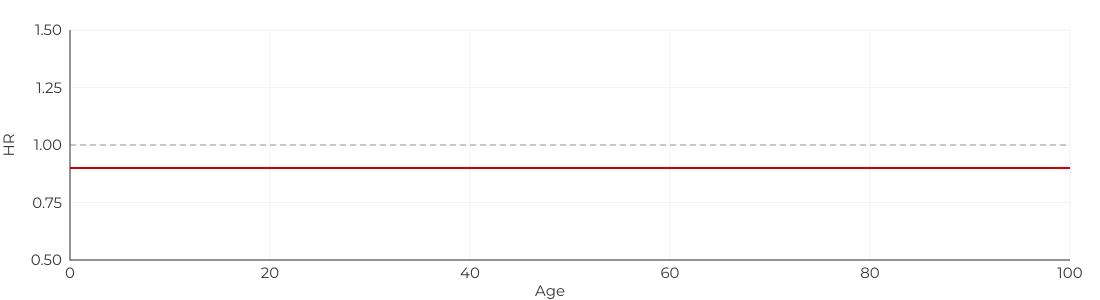
Here are the results:

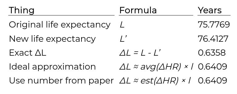
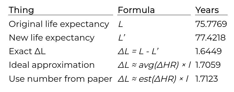
Let me explain what’s happening here. I made a simulator that takes actuarial data for how likely US males are to die at various ages. From this, it’s a simple spreadsheet calculation to compute life expectancy L.^[13] Then I applied a hazard ratio to change the probability of dying at each age, and re-ran the simulator to compute a new life expectancy L’ and the exact difference ΔL. Then I’m showing two approximations of ΔL: The first is the “ideal approximation” using avg(ΔHR), which I’m including mostly to show that my math is good. Finally, I’m showing the approximation you get if you actually fit a Cox proportional hazards model and use the resulting number in est(ΔHR). This corresponds to what you’d get if you plug in a number from a paper.

So, with the above constant hazard ratio HR = 0.90, both approximations are very good. This remains true if you switch to some other constant.

What if the hazard ratio varies? At first, you might think that something like this would be very problematic:

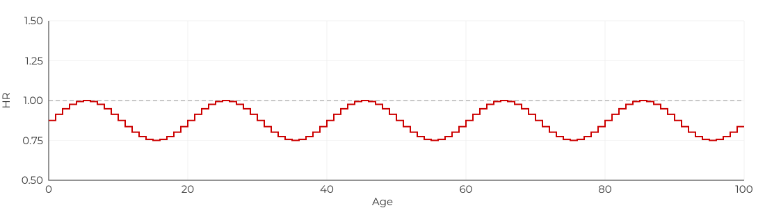
But it’s basically fine:

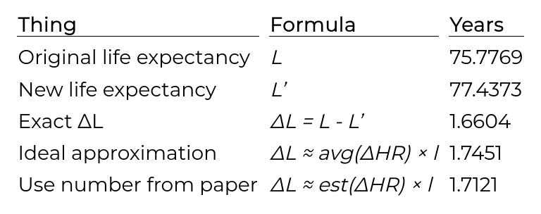
The reason this is fine is that the changes in the hazard ratio are relatively “high frequency”, meaning they sort of locally average out. To demonstrate this, suppose the hazard ratio is chosen randomly for each 1-year bin:

Then the approximations are even better:

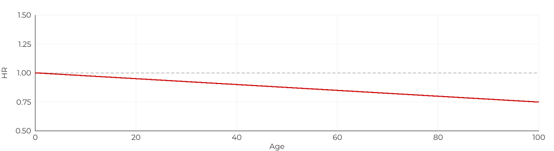
What causes trouble is if the hazard ratio varies systematically between the young and the old. For example, suppose the intervention is useless for newborns, but gradually becomes more helpful as you get older:

My “ideal approximation” would still be pretty accurate, if you could compute it. (Which you can’t, in the real world.) But using a number from a paper leads to an overestimate:

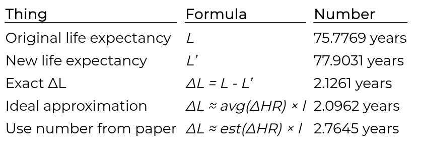
This happens because est(ΔHR) is implicitly weighted by P(t) which is heavily weighted towards older people, whereas we’d like to use something more like avg(ΔHR) which is weighted by P(t) × L(t) which is somewhat less weighted towards older people. Even so, the error isn’t terrible.

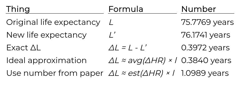
Now, it is possible that plugging in a hazard ratio from a paper could give wildly inaccurate estimates of life expectancy. One such scenario would be an intervention which is amazing for people aged 85-95, but does nothing for anyone else:

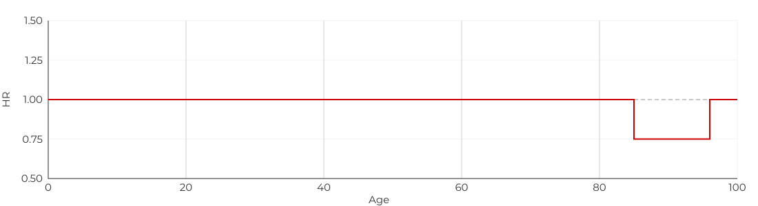
Now, the hazard ratio looks good exactly at the ages where est(ΔHR) has the most weight, leading it to hugely overestimate the impact on life expectancy:

Another nightmare case is an intervention that starts out harmful, but then switches to being helpful at older ages:

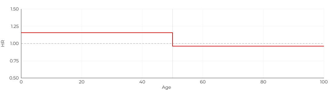
Now, using a number from a paper doesn’t even give an estimate with the right sign.

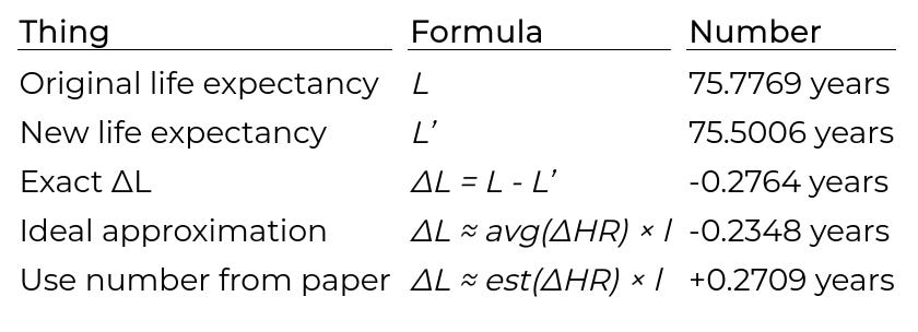
That’s bad. But I think most interventions probably aren’t like that? My guess is that most real interventions vary somewhat with age, but they do so gradually and without switching sign. In those cases, it’s quite difficult to find cases where plugging in the number from a paper is off by more than 30% or so. If you don’t believe me, just try it.^[14]

TLDR

If we were another species, it might be very hard to convert from hazard ratios to changes in life expectancy. But for modern people in rich countries, there are three lucky coincidences:

1. Mortality risk happens to be distributed so that you can approximate changes in life expectancy through a simple weighted sum of hazard ratios at different ages, ignoring interactions.

2. The statistical method that people use to estimate scalar hazard ratios can also be approximated as a weighted sum of hazard ratios at different ages, ignoring interactions.

3. The weights that you need to estimate life expectancy (from #1) and the weights that are implicitly used to compute hazard ratio numbers (from #2) aren’t the same. But they’re fairly close.

These facts justify taking an estimated hazard ratio number HR from a paper and approximating the change in life expectancy as ΔL ≈ ln(1/HR) × 12.93 years or, if the hazard ratio is close to one and you hate logarithms, as ΔL ≈ (1-HR) × 12.93 years.

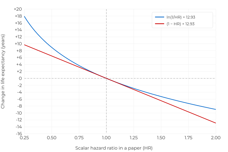
The number 12.93 years is for US males. It’s the product of Keyfitz entropy (0.17) and baseline life expectancy (75.8 years). It will vary a bit in other populations.

If the true underlying hazard ratio:

• …is constant across ages, then the above approximation will be extremely good.

• …decreases as people get older, that approximation will overestimate ΔL. That is, it will make helpful interventions look better than they actually are, and it will make harmful interventions look less bad than they actually are.

• …increases as people get older, that approximation will underestimate ΔL. That is, it will make helpful interventions look less good than they actually are, and it will make harmful interventions look worse than they actually are.

But as long as the true underlying hazard ratio isn’t too crazy, there’s probably not more than ~30% error in either direction.

Finally, two major caveats: First, the above discussion assumes that the hazard ratio was estimated by running a trial on people of all ages. In general, est(ΔHR) implicitly gives weight to different ages proportional to how many deaths occur at those ages in the baseline population in the trial. If there’s a minimum age of, say, 50 years old, that won’t change too much because most of the mass of P(t) is above the age of 50 anyway. But if there’s a minimum age of 70, or a maximum age of 50, that could make a huge difference if the true hazard ratio is different at the ages that weren’t seen.

Second, these are estimates for the life expectancy for a population. But you are not a population. In some sense, your genetics and lifestyle mean you have your own “personal Keyfitz entropy”, reflecting how spread out your mortality would be for you if you led millions random lives. If you drive safely and use an air purifier and eat well and get exercise and don’t smoke, that likely means your personal life expectancy is higher than average. But it also probably means that your personal Keyfitz entropy is lower than average.^[15] So, if you make your lifestyle even better by eating more fiber or whatever, even if that produces the same hazard ratio for you as for other people, it would still likely lead to smaller increases in life expectancy, for the same reason that the same hazard ratio produces smaller changes in lifespan in humans compared to mice. What we really need is some interventions strong enough to break the math behind these approximations and free us from Keyfitz tyranny.

---

1. 

   ↩︎

2. I know, I know, you care about quality of life, not just years of life. I agree, some number that measures health and vitality, maybe disability-adjusted life years or quality-adjusted life years, would be better. But these are hard to estimate and so are rarely reported. Anyway, in practice most interventions that make you more vital tend to make you live longer and vice versa, so focusing on life expectancy isn’t too bad.↩︎

3. In this model, the number of days of life follows a geometric distribution with p = (number of bullets) / (number of chambers). So the mean life expectancy is 1/p days or (number of chambers) / (number of bullets) days. With 54,786 chambers and 2 bullets, that works out to 75 years. And if you drop down to one bullet, then it increases to 150 years.↩︎

4. If some intervention would have reduce mortality among people aged ≥ 60 in prehistorical tribal bands, that wouldn’t have increased life expectancy very much, because most people didn’t make it to 60. But compared to prehistorical tribal bands, we have in fact vastly reduced mortality at younger ages. And so, today, reducing mortality for people aged ≥ 60 will increase life expectancy a lot.↩︎

5. You might think this is stupid. Why change a relative risk into a hazard ratio if you’re just going to assume it’s constant? Isn’t that pointless? Well, no. Remember how relative risks always go to 1.0 for long enough trials as everyone in both the treatment and control groups departs our coil? That doesn’t happen with constant hazard ratios.↩︎

6. It’s usually (though not always) better to use ΔHR(t) = ln(1/HR(t)). This correctly reflects, for example, that if all hazard ratios go to zero, then life expectancy goes to infinity, yay. These two approximations are almost identical for hazard ratios that are close to one because ln(1/r) ≈ (1-r) when r is close to one. So if you are terrified of logarithms but you’ve made it to the end of this footnote anyway, you’re not missing out on too much.↩︎

7. There’s a degree of circularity to this argument. It assumes that hazard ratios transfer better between species than changes in life expectancy. That might be true, but it would be an empirical / biological fact, not something that’s guaranteed by logic.↩︎

8. To see this, note that ΔL ≈ ∑ₜ ΔHR(t) × P(t) × L(t) = L̄ × ∑ₜ ΔHR(t) × (P(t) × L(t) / L̄) = L̄ × avg(ΔHR).↩︎

9. A pretty decent approximation turns out to be

   avg(ΔHR) ≈ 0.27 × avg₂₀₋₅₀(ΔHR) + 0.73 × avg₅₀₋₉₀(ΔHR),

   where avg₂₀₋₅₀(ΔHR) represents a flat average of the change over the ages 20 to 50 and avg₅₀₋₉₀(ΔHR) represents a flat average over the ages 50 to 90.↩︎

10. That is, it’s better to use est(ΔHR) = ln(1/est(HR)). This is close to 1-est(HR) when est(HR) is close to one.↩︎

11. If there is an infinite amount of data, the typical method reduces to solving

    ∑ₜ (P(t) + P’(t)) × π(t, HR) = ∑ₜ P’(t),

    for HR. Here, P’(t) is the chance of dying at age t after the hazard ratio has been applied, and π(t, HR) is the probability that, if a death occurred at time t, it was in the treatment group. Of course, the true probability that a death is in the treatment group is P’(t) / (P(t) + P’(t)). The standard “proportional Cox” model assumes that the hazard ratio is constant and so replaces this raw fraction with a model-based one, namely

    π(t, HR) = S’(t) × HR / (S(t) + S’(t) × HR).

    This reflects the fact that at age t, a fraction S(t) of controls are alive and each of these have some chance μ(t) of dying, so P(t)=S(t) × μ(t). Meanwhile, a fraction S’(t) of the treatment group is alive, and these each have a chance HR × μ(t) of dying, meaning that P’(t) = S’(t) × HR × μ(t). If you substitute these equations for P(t) and P’(t) into the second equation above, the factor of μ(t) conveniently cancels and you get π(t, HR) as written.

    In effect, the hazard ratio’s job is to attribute deaths to the treatment versus the control group. Now, if the true time-varying HR(t) is close to one, then it can be shown that the estimated hazard ratio est(HR) approximately satisfies

    ln(est(HR)) ≈ ∑ₜ P(t) ln(HR(t)).↩︎

12. The geometric average is equivalent to the condition that

    ln(est(HR)) ≈ ∑ₜ P(t) ln(HR(t))

    Using the “better” approximation that ΔHR(t) = ln(1/HR(t)) and *est(ΔHR)=ln(1/est(HR)), it follows that

    est(ΔHR) ≈ ∑ₜ P(t) ΔHR(t).

    You can justify interpreting that same equation using est(ΔHR) = 1-est(HR) and ΔHR(t)=1-HR(t) from the fact that these are almost the same when HR(t) is close to one.↩︎

13. This simulator pretends that people live for integer numbers of years. That’s not true in reality, of course, but it makes the simulator easier to implement and understand and makes little difference in practice.↩︎

14. In the simulation, “true ΔL” is what I called “exact ΔL” above, while “approximation (log)” is what I called “ideal approximation” and “Cox fitted” is what I called “Use number from paper”.↩︎

15. The way modern human mortality is distributed, even if your healthy lifestyle were to reduce mortality by a constant factor at all ages, that still has the effect of decreasing Keyfitz entropy.↩︎